Title

Einführung in die Technische Informatik
Prof. Jian-Jia Chen | Dr.-Ing. Christian Hakert | Dr. rer. nat. Marcus Völker
RWTH Aachen University

Kapitel 3: Vereinfachung Boolescher Funktionen

Vereinfachung Boolescher Funktionen

Resolutionsregel: \(\quad ab\lor a\overline{b}=a(b\lor \overline{b})=a\land 1=a\)

Beispiel 1:

\[ \begin{aligned} f(x_2,x_1,x_0) &= \overline{x_2}x_1x_0\lor x_2x_1x_0\\ &= (\overline{x_2}\lor x_2)x_1x_0\\ &= x_1x_0 \end{aligned} \]

Beispiel 2:

\[ \begin{aligned} f(x_3,x_2,x_1,x_0) &= x_3\overline{x_2}x_1x_0\lor x_3\overline{x_2}\,\overline{x_1}x_0\lor x_3x_2x_1x_0\lor \overline{x_3}\,\overline{x_2}\,\overline{x_1}x_0\lor \overline{x_3}\,\overline{x_2}x_1x_0\\ &= x_3\overline{x_2}x_0\lor x_3x_1x_0\lor \overline{x_2}\,\overline{x_1}x_0\lor \overline{x_3}\,\overline{x_2}x_0\lor \overline{x_2}x_1x_0\\ &= \overline{x_2}x_0\lor x_3x_1x_0 \end{aligned} \]

Minimalpolynom

  • Polynom = DF = Sum of products (SoP)
  • Sei \(M\) ein Polynom für \(f:B^n\to B^1\)
  • \(M\) heißt Minimalpolynom (für \(f\)), wenn es kein Polynom geringerer Länge für \(f\) gibt.
  • Die Länge eines Polynoms ist definiert als die Anzahl der Literale, die es enthält

Abschnitt 3.1

OBDDs und Vereinfachung

  • Grundoperationen zur Vereinfachung von OBDDs
  • Relevanz der Variablenordnung

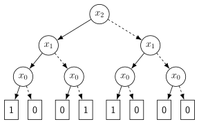
Wiederholung: Funktion als Entscheidungsbaum

\(x_2\) \(x_1\) \(x_0\) \(f\)
0 0 0 0
0 0 1 0
0 1 0 0
0 1 1 1
1 0 0 1
1 0 1 0
1 1 0 0
1 1 1 1
ti-3-deck-code-7441145a.tex.svg

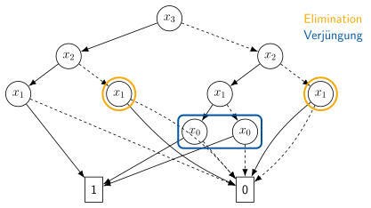
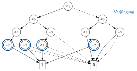
1. Grundoperation zur Vereinfachung von OBDDs: Verjüngung (4-3 Regel)
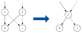
ti-3-deck-code-bb2f6a7d.tex.svg
  • Zwei Knoten mit derselben Variable und denselben Nachfolgern (1-Kante und 0-Kante) werden zu einem Knoten zusammengelegt.
  • Alle eingehenden Kanten zeigen danach auf den verbleibenden Knoten.

1. Grundoperation zur Vereinfachung von OBDDs: Verjüngung (4-3 Regel)
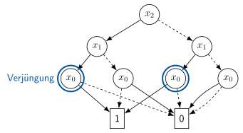
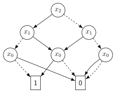
ti-3-deck-code-109003fc.tex.svg
  • Die beiden markierten \(x_0\)-Knoten haben dieselben Nachfolger und werden zusammengelegt.

1. Grundoperation zur Vereinfachung von OBDDs: Verjüngung (4-3 Regel)
ti-3-deck-code-dcdf8a68.tex.svg

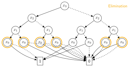
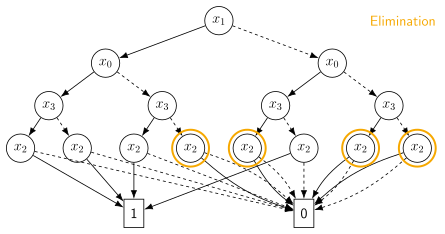
2. Grundoperation zur Vereinfachung von OBDDs: Elimination (2-1 Regel)
ti-3-deck-code-2579b728.tex.svg
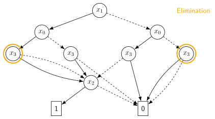
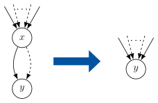
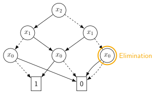
  • Zeigen beide ausgehenden Kanten eines Knotens auf denselben Nachfolger, ist der Test überflüssig: der Knoten wird entfernt.
  • Alle eingehenden Kanten zeigen danach direkt auf den Nachfolger.

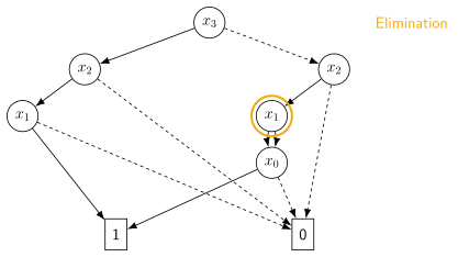
2. Grundoperation zur Vereinfachung von OBDDs: Elimination (2-1 Regel)
ti-3-deck-code-92f62ac4.tex.svg

2. Grundoperation zur Vereinfachung von OBDDs: Elimination (2-1 Regel)
ti-3-deck-code-8bc33301.tex.svg
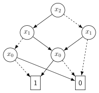
  • Das OBDD ist nun reduziert: keine der beiden Regeln ist mehr anwendbar.

Beispiel für OBDD (Variablenordnung \(x_3<x_2<x_1<x_0\))

\[ f(x_3,x_2,x_1,x_0)=x_3x_2x_1x_0\lor \overline{x_3}x_2x_1x_0\lor x_3x_2x_1\overline{x_0}\lor \overline{x_3}x_2\overline{x_1}x_0 \]
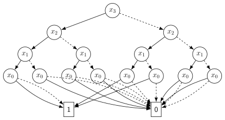
ti-3-deck-code-4fd81cfd.tex.svg

Beispiel für OBDD: Schritt 1

ti-3-deck-code-54563366.tex.svg

Beispiel für OBDD: Schritt 2

ti-3-deck-code-ccce36c1.tex.svg

Beispiel für OBDD: Schritt 3

ti-3-deck-code-3422d00d.tex.svg

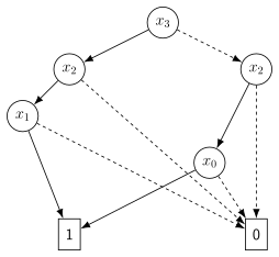
Reduziertes OBDD (Variablenordnung \(x_3<x_2<x_1<x_0\))
ti-3-deck-code-c8c63193.tex.svg

\(\Rightarrow\) Nicht weiter reduzierbar!

\[ f=x_3x_2x_1\lor \overline{x_3}x_2x_0 \]

Beispiel für OBDD (Variablenordnung \(x_1<x_0<x_3<x_2\))

\[ f(x_3,x_2,x_1,x_0)=x_3x_2x_1x_0\lor \overline{x_3}x_2x_1x_0\lor x_3x_2x_1\overline{x_0}\lor \overline{x_3}x_2\overline{x_1}x_0 \]
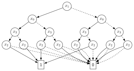
ti-3-deck-code-6289a470.tex.svg

Beispiel für OBDD: Schritt 1

ti-3-deck-code-f9ef7c4e.tex.svg

Beispiel für OBDD: Schritt 2

ti-3-deck-code-958a45c4.tex.svg

Beispiel für OBDD: Schritt 3

ti-3-deck-code-0722bfae.tex.svg

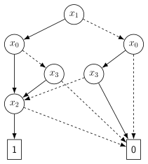
Reduziertes OBDD (Variablenordnung \(x_1<x_0<x_3<x_2\))
ti-3-deck-code-1f2ec937.tex.svg

\(\Rightarrow\) Nicht weiter reduzierbar!

\[ f=x_2x_1x_0\lor x_3x_2x_1\overline{x_0}\lor \overline{x_3}x_2\overline{x_1}x_0 \]

Vergleich der Variablenordnung

Variablenordnung Resultat
OBDD (Variablenordnung \(x_3<x_2<x_1<x_0\)) \(f=x_3x_2x_1\lor \overline{x_3}x_2x_0\)
OBDD (Variablenordnung \(x_1<x_0<x_3<x_2\)) \(f=x_2x_1x_0\lor x_3x_2x_1\overline{x_0}\lor \overline{x_3}x_2\overline{x_1}x_0\)
  • Reduziertes OBDD: 5 statt 6 innere Knoten

\(\Rightarrow\) Variablenordnung bei OBDDs relevant!

Abschnitt 3.2

Karnaugh-Diagramme

  • Implikanten
  • Don’t Cares

Wiederholung: Karnaugh-Diagramme für n = 2
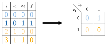
ti-3-deck-code-1b4b43d0.tex.svg

Wiederholung: Karnaugh-Diagramme für n = 3, 4
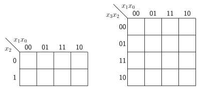
ti-3-deck-code-9b41d08a.tex.svg

Blockbildung

  • Blöcke müssen maximale Größe haben
  • Die Blockgröße muss eine Zweierpotenz sein
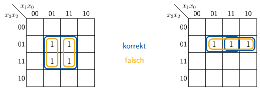
ti-3-deck-code-bcfe7154.tex.svg

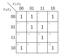
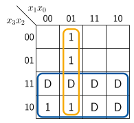
Beispiel

\[ f(x_3,x_2,x_1,x_0)=x_3\overline{x_2}x_1x_0\lor x_3\overline{x_2}\,\overline{x_1}x_0\lor x_3x_2x_1x_0\lor \overline{x_3}\,\overline{x_2}\,\overline{x_1}x_0\lor \overline{x_3}\,\overline{x_2}x_1x_0 \]
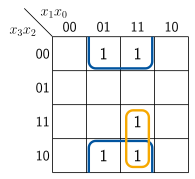
ti-3-deck-code-8fdda352.tex.svg
  • Blau: \(\overline{x_2}x_0\) (Block über den Rand)
  • Orange: \(x_3x_1x_0\)

Vereinfachte Form:

\[ f=\overline{x_2}x_0\lor x_3x_1x_0 \]

Beispiel

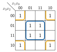
\[ \begin{aligned} f={}&\overline{x_3}\,\overline{x_2}\,\overline{x_1}\,\overline{x_0}\lor x_3\overline{x_2}\,\overline{x_1}\,\overline{x_0}\lor \overline{x_3}x_2\overline{x_1}x_0\lor x_3x_2\overline{x_1}x_0\\ &\lor \overline{x_3}x_2x_1x_0\lor x_3x_2x_1x_0\lor \overline{x_3}\,\overline{x_2}x_1\overline{x_0}\lor x_3\overline{x_2}x_1\overline{x_0} \end{aligned} \]
ti-3-deck-code-5084d1bf.tex.svg
  • Blau: \(x_2x_0\)
  • Orange: \(\overline{x_2}\,\overline{x_0}\) (die vier Ecken bilden einen Block)

Vereinfachte Form:

\[ f=x_2x_0\lor \overline{x_2}\,\overline{x_0} \]

Definition

Sei \(f:B^n\to B\) eine Boolesche Funktion. Ein Term \(M\neq 0\) heißt Implikant von \(f\), kurz \(M\leq f\), falls \(M(x)\leq f(x)\) für alle \(x\in B^n\) gilt, d.h.

\[ M(x)=1\Rightarrow f(x)=1 \qquad \forall x\in B^n \]

Ein Implikant \(M\) von \(f\) heißt Primimplikant (von \(f\)), falls keine echte Verkürzung von \(M\) noch Implikant von \(f\) ist.

Ein Primimplikant \(M\) heißt Kernimplikant (von \(f\)), falls \(M\) in jedem Minimalpolynom von \(f\) vorkommt.

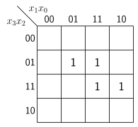
Beispiel 2

\[ f=x_3x_2x_1x_0\lor \overline{x_3}x_2x_1x_0\lor x_3x_2x_1\overline{x_0}\lor \overline{x_3}x_2\overline{x_1}x_0 \]
ti-3-deck-code-2b3dc550.tex.svg

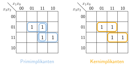
Beispiel 2

\[ f=x_3x_2x_1x_0\lor \overline{x_3}x_2x_1x_0\lor x_3x_2x_1\overline{x_0}\lor \overline{x_3}x_2\overline{x_1}x_0 \]
ti-3-deck-code-60fc585a.tex.svg
  • Primimplikanten: \(\overline{x_3}x_2x_0,\ x_2x_1x_0,\ x_3x_2x_1\)
  • Kernimplikanten: \(\overline{x_3}x_2x_0,\ x_3x_2x_1\) \(\Rightarrow\) Minimalpolynom \(f=x_3x_2x_1\lor \overline{x_3}x_2x_0\)

KV-Kochrezept

  1. Wertetabelle
  2. Einsen ins KV-Diagramm
  3. Alle Primimplikanten: maximale Blöcke
  4. Minimale Überdeckung \(\Rightarrow\) Minimalpolynom

KV-Kochrezept: 0. Wertetabelle

\(i\) \(x_3\) \(x_2\) \(x_1\) \(x_0\) \(f\)
0 0 0 0 0 1
1 0 0 0 1 1
2 0 0 1 0 1
3 0 0 1 1 0
4 0 1 0 0 0
5 0 1 0 1 1
6 0 1 1 0 0
7 0 1 1 1 1
\(i\) \(x_3\) \(x_2\) \(x_1\) \(x_0\) \(f\)
8 1 0 0 0 1
9 1 0 0 1 0
10 1 0 1 0 1
11 1 0 1 1 0
12 1 1 0 0 0
13 1 1 0 1 0
14 1 1 1 0 0
15 1 1 1 1 1

KV-Kochrezept: 1. Einsen eintragen

ti-3-deck-code-0204f26d.tex.svg
  • Nullen weglassen

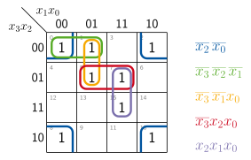
KV-Kochrezept: 2. Alle Primimplikanten
ti-3-deck-code-8d000173.tex.svg
  • Blöcke maximal, Größe \(2^k\), auch über den Rand

KV-Kochrezept: 3. Minimale Überdeckung
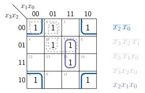
ti-3-deck-code-d64b454a.tex.svg
  • Einsen mit nur einem Block \(\Rightarrow\) Kernimplikant

KV-Kochrezept: 3. Minimale Überdeckung
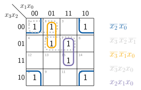
ti-3-deck-code-86a6d23a.tex.svg
  • Restliche Einsen mit möglichst wenigen Blöcken

\[ f=\overline{x_2}\,\overline{x_0}\lor x_2x_1x_0\lor \overline{x_3}\,\overline{x_1}x_0 \]

Ausnutzung von Don’t Cares

\(x\) \(x_3\) \(x_2\) \(x_1\) \(x_0\) \(f\)
0 0 0 0 0 0
1 0 0 0 1 1
2 0 0 1 0 0
3 0 0 1 1 0
4 0 1 0 0 0
5 0 1 0 1 1
6 0 1 1 0 0
7 0 1 1 1 0
8 1 0 0 0 1
9 1 0 0 1 1
A 1 0 1 0 D
B 1 0 1 1 D
C 1 1 0 0 D
D 1 1 0 1 D
E 1 1 1 0 D
F 1 1 1 1 D
  • Eingaben A–F kommen nicht vor (z.B. BCD-Code)
  • D (Don’t Care): Funktionswert beliebig, kann zu 0 oder 1 gewählt werden
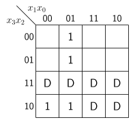
ti-3-deck-code-d74373bc.tex.svg

Ausnutzung von Don’t Cares

ti-3-deck-code-7aeee048.tex.svg
  • Don’t Cares werden als 1 behandelt, wo sie größere Blöcke ermöglichen
  • Blau: \(x_3\), Orange: \(\overline{x_1}x_0\)

Ergebnis: \(\quad f(x_3,x_2,x_1,x_0)=x_3\lor \overline{x_1}x_0\)

Abschnitt 3.3

Quine-McCluskey-Verfahren

  • Bestimmung der Primimplikanten
  • Implikationsmatrix
  • Mehrdeutigkeit von Minimalpolynomen

Motivation: KV-Diagramm für 6 Variablen

Quine-McCluskey-Verfahren: Vorgehen

  1. Minterme der einschlägigen Indizes nach Anzahl der Negationen gruppieren
  2. Resolutionsregel \(ab\lor a\overline{b}=a\) auf Terme benachbarter Gruppen anwenden, solange möglich
  3. Terme, die sich nicht weiter verkürzen lassen, sind die Primimplikanten
  4. Implikationsmatrix aufstellen: Welcher Primimplikant deckt welchen Minterm ab?
  5. Kernimplikanten wählen, restliche Minterme mit möglichst kurzen Primimplikanten abdecken

Quine-McCluskey-Verfahren

\[ \begin{aligned} f={}&\overline{x_3}\,\overline{x_2}\,\overline{x_1}\,\overline{x_0}\lor \overline{x_3}x_2\overline{x_1}\,\overline{x_0}\lor \overline{x_3}x_2x_1\overline{x_0}\lor x_3\overline{x_2}x_1x_0\\ &\lor x_3x_2\overline{x_1}\,\overline{x_0}\lor x_3x_2\overline{x_1}x_0\lor x_3x_2x_1\overline{x_0} \end{aligned} \]

Minterme gemäß Anzahl der Negationen:

Gruppe Implikant Index (dezimal)
1 \(x_3\overline{x_2}x_1x_0\) 11
\(x_3x_2\overline{x_1}x_0\) 13
\(x_3x_2x_1\overline{x_0}\) 14
2 \(\overline{x_3}x_2x_1\overline{x_0}\) 6
\(x_3x_2\overline{x_1}\,\overline{x_0}\) 12
3 \(\overline{x_3}x_2\overline{x_1}\,\overline{x_0}\) 4
4 \(\overline{x_3}\,\overline{x_2}\,\overline{x_1}\,\overline{x_0}\) 0

Quine-McCluskey-Verfahren

Nach erster Anwendung der Resolutionsregel:

Gruppe Implikant Index (dezimal)
1 \(x_3\overline{x_2}x_1x_0\) 11
\(x_2x_1\overline{x_0}\) 6,14
\(x_3x_2\overline{x_1}\) 12,13
\(x_3x_2\overline{x_0}\) 12,14
2 \(\overline{x_3}x_2\overline{x_0}\) 4,6
\(x_2\overline{x_1}\,\overline{x_0}\) 4,12
3 \(\overline{x_3}\,\overline{x_1}\,\overline{x_0}\) 0,4

Alle Primimplikanten:

Gruppe Implikant Index (dezimal)
1 \(x_3\overline{x_2}x_1x_0\) 11
\(x_3x_2\overline{x_1}\) 12,13
\(x_2\overline{x_0}\) 4,6,12,14
3 \(\overline{x_3}\,\overline{x_1}\,\overline{x_0}\) 0,4

Quine-McCluskey-Verfahren

Implikationsmatrix:

Primimplikant \ Minterm 0 4 6 11 12 13 14
\(x_3\overline{x_2}x_1x_0\) 0 0 0 1 0 0 0
\(x_3x_2\overline{x_1}\) 0 0 0 0 1 1 0
\(x_2\overline{x_0}\) 0 1 1 0 1 0 1
\(\overline{x_3}\,\overline{x_1}\,\overline{x_0}\) 1 1 0 0 0 0 0

Kostengünstigste Darstellung:

\[ f=x_3\overline{x_2}x_1x_0\lor x_3x_2\overline{x_1}\lor x_2\overline{x_0}\lor \overline{x_3}\,\overline{x_1}\,\overline{x_0} \]

Beispiel zum Quine-McCluskey-Verfahren

Anderes Beispiel:

\[ \begin{aligned} f={}&x_3\overline{x_2}x_1x_0\lor x_3\overline{x_2}x_1\overline{x_0}\lor x_3\overline{x_2}\,\overline{x_1}\,\overline{x_0}\lor \overline{x_3}x_2x_1x_0\lor \overline{x_3}x_2x_1\overline{x_0}\\ &\lor \overline{x_3}x_2\overline{x_1}x_0\lor \overline{x_3}x_2\overline{x_1}\,\overline{x_0}\lor \overline{x_3}\,\overline{x_2}x_1x_0\lor \overline{x_3}\,\overline{x_2}\,\overline{x_1}\,\overline{x_0} \end{aligned} \]

Minterme gemäß Anzahl der Negationen:

Gruppe Implikant Index (dezimal)
1 \(\overline{x_3}x_2x_1x_0\) 7
\(x_3\overline{x_2}x_1x_0\) 11
2 \(\overline{x_3}\,\overline{x_2}x_1x_0\) 3
\(\overline{x_3}x_2\overline{x_1}x_0\) 5
\(\overline{x_3}x_2x_1\overline{x_0}\) 6
\(x_3\overline{x_2}x_1\overline{x_0}\) 10
3 \(\overline{x_3}x_2\overline{x_1}\,\overline{x_0}\) 4
\(x_3\overline{x_2}\,\overline{x_1}\,\overline{x_0}\) 8
4 \(\overline{x_3}\,\overline{x_2}\,\overline{x_1}\,\overline{x_0}\) 0

Beispiel zum Quine-McCluskey-Verfahren

Nach erster Anwendung der Resolutionsregel:

Gruppe Implikant Index (dezimal)
1 \(\overline{x_3}x_1x_0\) 3,7
\(\overline{x_3}x_2x_0\) 5,7
\(\overline{x_3}x_2x_1\) 6,7
\(\overline{x_2}x_1x_0\) 3,11
\(x_3\overline{x_2}x_1\) 10,11
2 \(\overline{x_3}x_2\overline{x_1}\) 4,5
\(\overline{x_3}x_2\overline{x_0}\) 4,6
\(x_3\overline{x_2}\,\overline{x_0}\) 8,10
3 \(\overline{x_3}\,\overline{x_1}\,\overline{x_0}\) 0,4
\(\overline{x_2}\,\overline{x_1}\,\overline{x_0}\) 0,8

Nach zweiter Anwendung der Resolutionsregel:

Gruppe Implikant Index (dezimal)
1 \(\overline{x_3}x_1x_0\) 3,7
\(\overline{x_3}x_2\) 4,5,6,7
\(\overline{x_2}x_1x_0\) 3,11
\(x_3\overline{x_2}x_1\) 10,11
2 \(x_3\overline{x_2}\,\overline{x_0}\) 8,10
3 \(\overline{x_3}\,\overline{x_1}\,\overline{x_0}\) 0,4
\(\overline{x_2}\,\overline{x_1}\,\overline{x_0}\) 0,8

Keine weitere Anwendung mehr möglich

Beispiel zum Quine-McCluskey-Verfahren

Implikationsmatrix:

Primimplikant \ Minterm 0 3 4 5 6 7 8 10 11
\(\overline{x_3}x_1x_0\) 0 1 0 0 0 1 0 0 0
\(\overline{x_3}x_2\) 0 0 1 1 1 1 0 0 0
\(\overline{x_2}x_1x_0\) 0 1 0 0 0 0 0 0 1
\(x_3\overline{x_2}x_1\) 0 0 0 0 0 0 0 1 1
\(x_3\overline{x_2}\,\overline{x_0}\) 0 0 0 0 0 0 1 1 0
\(\overline{x_3}\,\overline{x_1}\,\overline{x_0}\) 1 0 1 0 0 0 0 0 0
\(\overline{x_2}\,\overline{x_1}\,\overline{x_0}\) 1 0 0 0 0 0 1 0 0

Kernimplikant: \(\overline{x_3}x_2\) (einziger Primimplikant für die Minterme 5 und 6)

Kostengünstigste Darstellung: Hier nicht eindeutig!

Beispiel zum Quine-McCluskey-Verfahren

Mögliche Minimalpolynome (jeweils mit Kernimplikant \(\overline{x_3}x_2\)):

\[ \begin{aligned} f_1 &= \overline{x_3}x_2\lor \overline{x_2}x_1x_0\lor x_3\overline{x_2}x_1\lor \overline{x_2}\,\overline{x_1}\,\overline{x_0}\\ f_2 &= \overline{x_3}x_2\lor \overline{x_2}x_1x_0\lor x_3\overline{x_2}\,\overline{x_0}\lor \overline{x_2}\,\overline{x_1}\,\overline{x_0}\\ f_3 &= \overline{x_3}x_2\lor \overline{x_3}x_1x_0\lor x_3\overline{x_2}x_1\lor \overline{x_2}\,\overline{x_1}\,\overline{x_0}\\ f_4 &= \overline{x_3}x_2\lor \overline{x_2}x_1x_0\lor x_3\overline{x_2}\,\overline{x_0}\lor \overline{x_3}\,\overline{x_1}\,\overline{x_0} \end{aligned} \]

  • Alle vier Polynome haben die Länge 11.

Beispiel zum Quine-McCluskey-Verfahren

Kernimplikant \(\overline{x_3}x_2\) gewählt \(\Rightarrow\) Minterme 4, 5, 6, 7 sind abgedeckt.

Primimplikant \ Minterm 0 3 8 10 11
\(\overline{x_3}x_1x_0\) 0 1 0 0 0
\(\boldsymbol{\overline{x_2}x_1x_0}\) 0 1 0 0 1
\(x_3\overline{x_2}x_1\) 0 0 0 1 1
\(x_3\overline{x_2}\,\overline{x_0}\) 0 0 1 1 0
\(\overline{x_3}\,\overline{x_1}\,\overline{x_0}\) 1 0 0 0 0
\(\overline{x_2}\,\overline{x_1}\,\overline{x_0}\) 1 0 1 0 0

Wähle beliebigen Implikanten mit neuer Information!

\[ f_1=\overline{x_3}x_2\lor \overline{x_2}x_1x_0 \]

Beispiel zum Quine-McCluskey-Verfahren

Minterme 3 und 11 sind nun ebenfalls abgedeckt.

Primimplikant \ Minterm 0 8 10
\(\overline{x_3}x_1x_0\) 0 0 0
\(x_3\overline{x_2}x_1\) 0 0 1
\(x_3\overline{x_2}\,\overline{x_0}\) 0 1 1
\(\overline{x_3}\,\overline{x_1}\,\overline{x_0}\) 1 0 0
\(\boldsymbol{\overline{x_2}\,\overline{x_1}\,\overline{x_0}}\) 1 1 0

Wähle beliebigen Implikanten mit neuer Information!

\[ f_1=\overline{x_3}x_2\lor \overline{x_2}x_1x_0\lor \overline{x_2}\,\overline{x_1}\,\overline{x_0} \]

Beispiel zum Quine-McCluskey-Verfahren

Nur noch Minterm 10 ist offen.

Primimplikant \ Minterm 10
\(\boldsymbol{x_3\overline{x_2}x_1}\) 1
\(x_3\overline{x_2}\,\overline{x_0}\) 1
\(\overline{x_3}\,\overline{x_1}\,\overline{x_0}\) 0

Wähle beliebigen Implikanten mit neuer Information!

\[ f_1=\overline{x_3}x_2\lor \overline{x_2}x_1x_0\lor \overline{x_2}\,\overline{x_1}\,\overline{x_0}\lor x_3\overline{x_2}x_1 \]

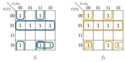
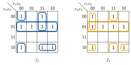
Mehrdeutigkeit am KV-Diagramm

ti-3-deck-code-9224e4b9.tex.svg

\[ \begin{aligned} f_1 &= \overline{x_3}x_2\lor \overline{x_2}x_1x_0\lor x_3\overline{x_2}x_1\lor \overline{x_2}\,\overline{x_1}\,\overline{x_0}\\ f_2 &= \overline{x_3}x_2\lor \overline{x_2}x_1x_0\lor x_3\overline{x_2}\,\overline{x_0}\lor \overline{x_2}\,\overline{x_1}\,\overline{x_0} \end{aligned} \]

Mehrdeutigkeit am KV-Diagramm
ti-3-deck-code-f4c5b78a.tex.svg

\[ \begin{aligned} f_3 &= \overline{x_3}x_2\lor \overline{x_3}x_1x_0\lor x_3\overline{x_2}x_1\lor \overline{x_2}\,\overline{x_1}\,\overline{x_0}\\ f_4 &= \overline{x_3}x_2\lor \overline{x_2}x_1x_0\lor x_3\overline{x_2}\,\overline{x_0}\lor \overline{x_3}\,\overline{x_1}\,\overline{x_0} \end{aligned} \]

Zusammenfassung

  • Warum minimieren?
    • Reduzierung von Eingangsvariablen und Schaltkreiselementen
    • Suche nach der optimalen Realisierung
  • In diesem Kapitel vorgestellt:

Definitionen

  • Minimalpolynom
  • (Prim- / Kern-) Implikant

Verfahren

  • (Reduzierte) OBDDs
  • Karnaugh-Veitch
  • Quine-McCluskey